Insights from Loan portfolio analysis for a FinTech loan product
 Photo by Franki Chamaki on Unsplash
Depending on business Key performance indicators, metrics that drive decisions can be obtained from loan data variables. Some of the key metrics include, but are not limited to, expected return, return rate, loan repayment ratio, actual returns/repayment, total amount overdue.
Overall, loan portfolio analysis is required when determining the ‘health’ of business. Accurate analysis of loan data will help make critical decisions that will support other departments’ operations, such as collections and customer support, and marketing.
This project entails an in-depth analysis of a fintech case loan product; datasets were obtained from a public domain. Given the dataset, different problems were addressed, and insights were obtained through analysis from the data.
Problems
- To understand from the data, the order at which subsequent customers purchased more than one product.
- Draw a pattern between the age of customers and products purchased.
- Repayment behavior measured with Timely Repayment Percentage (TRP) and the choice of product bought.
- Pattern between gender and choice of product bought.
- Length/number of days it takes for customers to fully repay their loans, addressing distribution and differences between the products.
- Given the products’ historical demand and repayment pattern, which one would you push for and why?
- The products demand trends over time.
- Which day(s) of the week has the highest loan repayment.
#load required packages
library(readxl)
library(dplyr)
library(tidyr)
library(lubridate)
library(ggplot2)
library(scales)
library(knitr)
#Read data
data <- read_excel("loan_data.xlsx")
data1.Order of products purchase by subsequent clients.
#Filter for only subsquent products, cycle greater than 1
summary <- data %>%
  filter(Cycle > 1) %>%
 select(Product,`Disbursed Date`,Cycle)
plot_data <- summary %>%
group_by(Product, Cycle) %>%
summarise(count = n())
plot_dataIn an analysis based on subsequent(repeat) customers, cycle 2 has the highest product demand. There was a high demand for BORA, LPG2, and CNVS in this cycle. BORA had a high number of purchases in cycle 2, then CNVS in cycle 3 and LPG2 in cycle 4. However, the difference is minimal, with an increase in number of cycles.
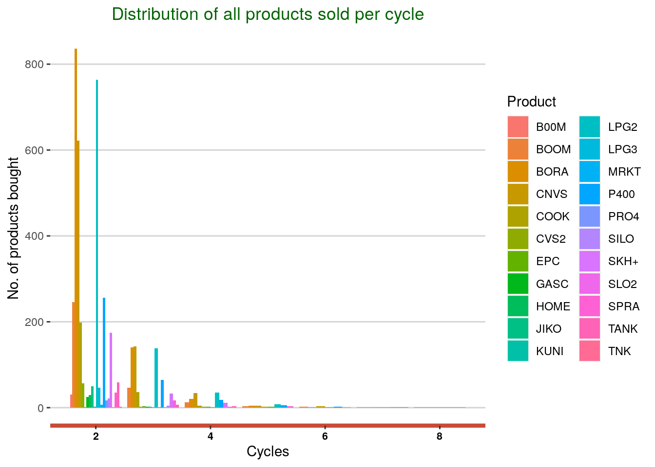
1.1 Displaying distribution for top products
For better visualization and clarity of the pattern, top products were filtered from the grouped product and cycles dataset.
Top_pdct <- plot_data %>%
  filter(Product=="BORA" | Product=="LPG2" | Product=="CNVS" | Product=="P400" | Product=="BOOM")
#display top rows and colums
head(Top_pdct)
## # A tibble: 6 x 3
## # Groups: Product [1]
## Product Cycle count
## <chr> <dbl> <int>
## 1 BOOM 2 246
## 2 BOOM 3 47
## 3 BOOM 4 12
## 4 BOOM 5 4
## 5 BOOM 6 2
## 6 BOOM 7 1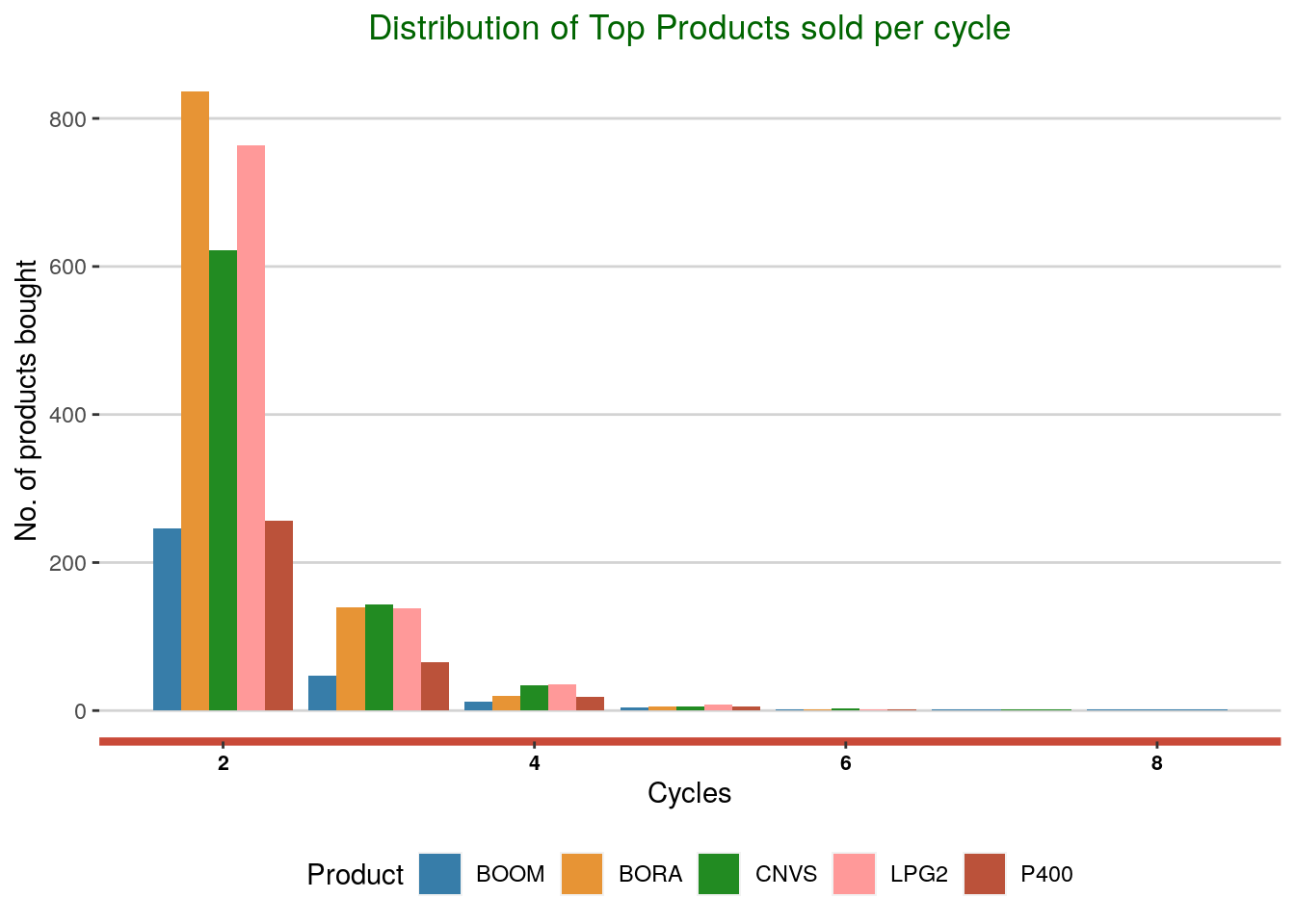
2.Relationships between age and product purchased
The Percentage age for each age group was computed from the sum of all purchases within the group.
Age_plot <- Age %>%
  group_by(Age, Product) %>%
  summarise(count = n())

#Percentage of product purchace per age
Percentage <- group_by(Age_plot, Age) %>%
  mutate(Percent = (count/sum(count))*100)

Percentage[,4] <- round(Percentage[,4], digits = 2)
#display top rows and columns
head(Percentage)## # A tibble: 6 x 4
## # Groups: Age [1]
## Age Product count Percent
## <dbl> <chr> <int> <dbl>
## 1 18 B00M 1 6.67
## 2 18 BORA 2 13.3
## 3 18 CNVS 1 6.67
## 4 18 LPG2 7 46.7
## 5 18 LPG3 2 13.3
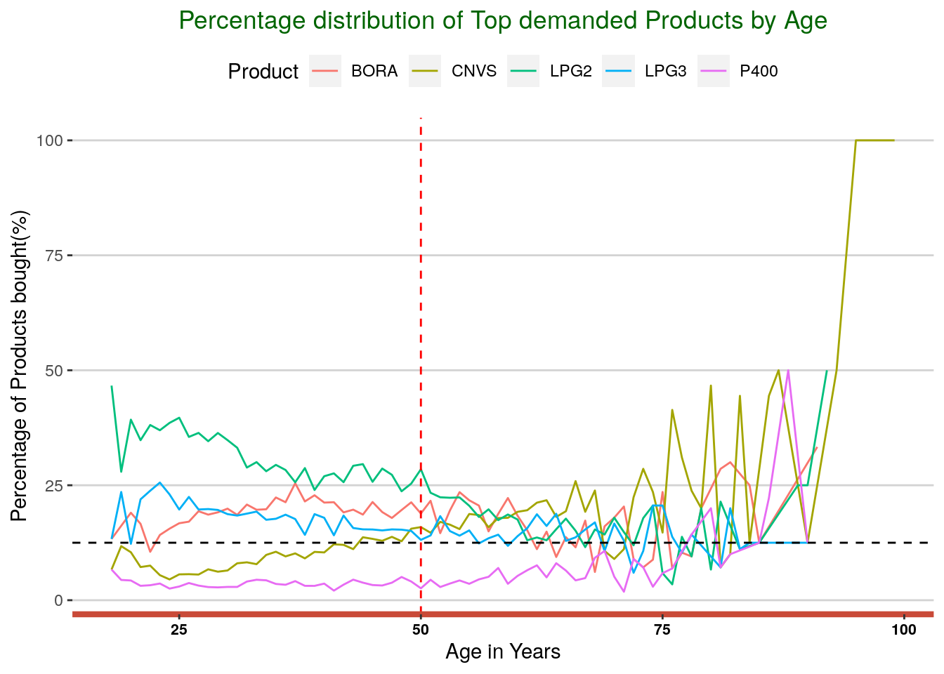
## 6 18 P400 1 6.67This data was used to show relationships between age and purchase of all products. The trend shows high age and products’ correlations in LPG2 and CNVS. There was a high demand for LPG2 between 18 and 50 years and a diminished demand in the age above 50 years with a less than 25% of the products purchased. On the other hand, CNVS was highly demanded by older age as compared to a younger age class. A pattern was observed in age, and this product demand; product demand increased with age.
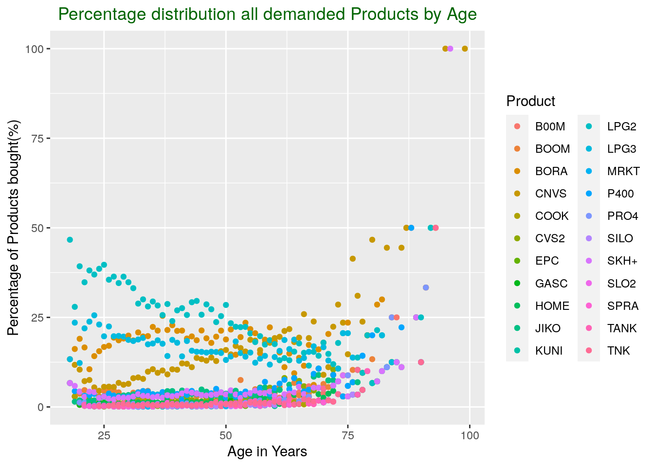
2.1 Age-products analysis for top demanded products
Top_Percent <- Percentage %>%
filter(Product=="CNVS" | Product=="LPG2" | Product=="LPG3" | Product=="BORA" | Product=="P400")
The trend line graph below explains in detail the relationship between age and products, as described above.
3. Repayment behaviour as measured with Timely Repayment Percentage(TRP) and choice of product bought
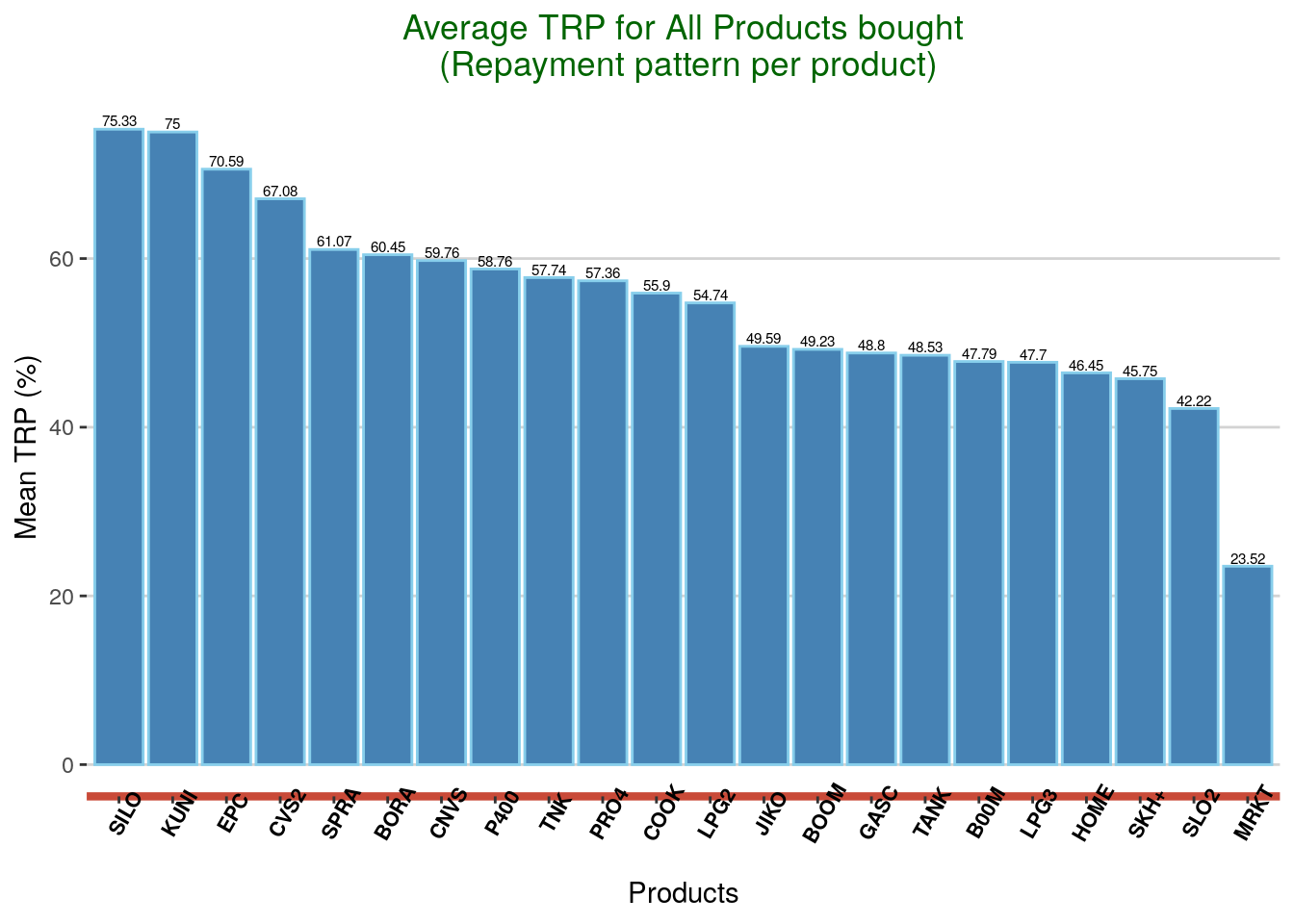
Average TRP for all products was used in this analysis.
TRP_summary <- group_by(TRP_clean, Product) %>%
summarise(mean(TRP)*100)
names(TRP_summary) <- c("Product", "Average_TRP")
TRP_summary[,2] <- round(TRP_summary[,2], digits = 2)head(TRP_summary)## # A tibble: 6 x 2
## Product Average_TRP
## <chr> <dbl>
## 1 B00M 47.8
## 2 BOOM 49.2
## 3 BORA 60.4
## 4 CNVS 59.8
## 5 COOK 55.9
## 6 CVS2 67.1Different products have a different measure of timely installment repayment ranging from 23.52% to 75.33%.In this case, the pattern shows SILOS and KUNI were more timely repaid compared to other products while MKRT had a low repayment frequency. 54% of the products (12/22) have a TRP of more than 50%.
4.Correlation/pattern between gender and choice of product bought
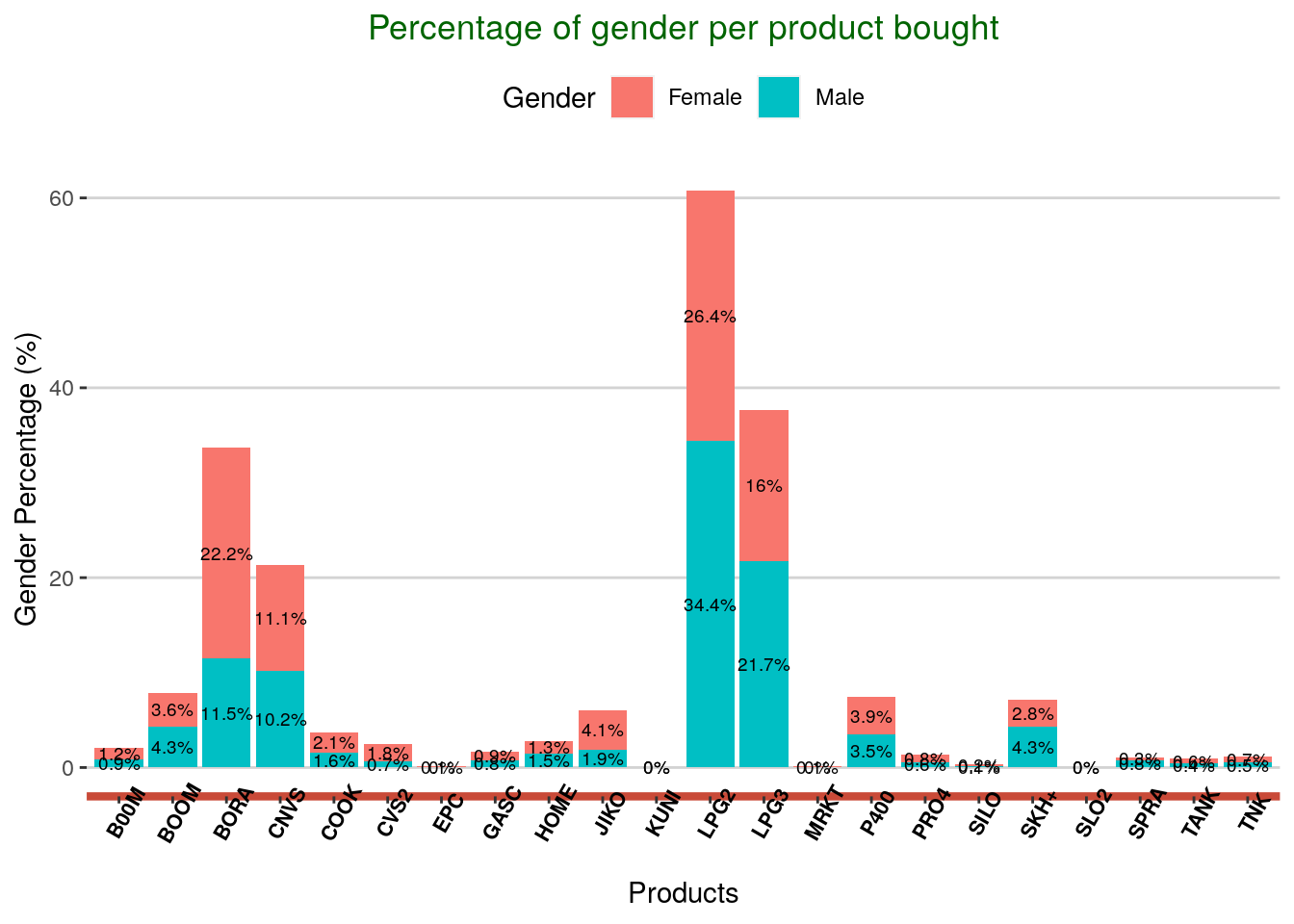
Percentage of gender to a specific product purchase was computed and used to derive the relationships between gender and products bought.
#create a gender dataset and add a percentage of gender purchase column
Gender_data <- data %>%
   group_by(Gender, Product) %>%
   summarize(count = n())

 Gender_summary <- group_by(Gender_data, Gender) %>%
   mutate(Percentage_gender =  (count/sum(count))*100)
 Gender_summary[,4] <- round(Gender_summary[,4], digits = 1)

 #Generate a plot dataset and position bar labels
 Gender_plot <- Gender_summary %>%
   group_by(Product) %>%
   arrange(Product, desc(Gender)) %>%
   mutate(lab_ypos = cumsum(Percentage_gender)- 0.5 * Percentage_gender)
The analysis shows most females dominated the products’ choice. However, four products: LPG2, LPG3, SKH+ and, BOOM were highly preferred by male.
5. Repayment length and distribution for full loan repayments
Full loan repayments here means: TRP = 100% and status = closed.
#Repayment data
 Repayments <- data %>%
     select(Product,`Disbursed Date`,Status,`Final Payment Date`, TRP) %>%
     filter(Status == "Closed" & TRP == 1.000)

Repayments$`Disbursed Date` <- as.Date(Repayments$`Disbursed Date`, format ="%Y-%m-%d")
 Repayments$`Final Payment Date` <- as.Date(Repayments$`Final Payment Date`, format = "%Y-%m-%d")

 #Add days column
 Repayments <-  mutate(Repayments, Days = as.numeric(`Final Payment Date` - `Disbursed Date`))
 #dispaly top rows and columns
head(Repayments)
## # A tibble: 6 x 6
## Product `Disbursed Date` Status `Final Payment Date` TRP Days
## <chr> <date> <chr> <date> <dbl> <dbl>
## 1 BORA 2019-01-09 Closed 2019-03-12 1 62
## 2 BORA 2019-01-09 Closed 2019-08-01 1 204
## 3 BORA 2019-01-09 Closed 2019-06-08 1 150
## 4 LPG2 2019-01-09 Closed 2019-05-01 1 112
## 5 LPG2 2019-01-09 Closed 2019-04-29 1 110
## 6 LPG2 2019-01-09 Closed 2019-05-06 1 117Most loans took around 110-120 days to be repaid fully.
## `stat_bin()` using `bins = 30`. Pick better value with `binwidth`.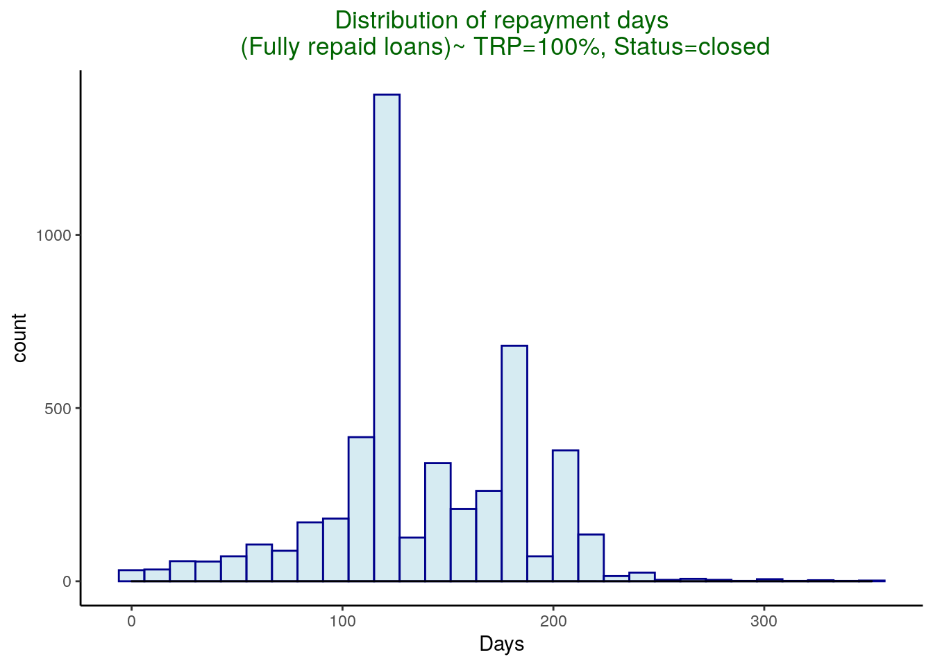
5.1 Distribution of timely full repaid loans per product.
To accurately know how long it took one product loan to be fully repaid and avoid bias, the mean of the days it took the products to be repaid was computed.
#Compute mean of products per group
mean_Repayment <- group_by(Repayments, Product) %>%
   mutate(Mean_days = mean(Days))
  mean_Repayment[, 7] <- trunc(mean_Repayment[, 7])

#dispaly top rows and columns
head(mean_Repayment)
## # A tibble: 6 x 7
## # Groups: Product [2]
## Product `Disbursed Date` Status `Final Payment Date` TRP Days Mean_days
## <chr> <date> <chr> <date> <dbl> <dbl> <dbl>
## 1 BORA 2019-01-09 Closed 2019-03-12 1 62 175
## 2 BORA 2019-01-09 Closed 2019-08-01 1 204 175
## 3 BORA 2019-01-09 Closed 2019-06-08 1 150 175
## 4 LPG2 2019-01-09 Closed 2019-05-01 1 112 110
## 5 LPG2 2019-01-09 Closed 2019-04-29 1 110 110
## 6 LPG2 2019-01-09 Closed 2019-05-06 1 117 110CNVS, COOK, CVS2, KUNI, LPG2, MKRT, and P400 were among the products with less timely repayment days(less than 120 days).
6.Historical demand and repayment behavior
Question: Which product would you push, and why? To better understand all products’ repayment behavior, the percentage of each product loan status was analyzed.For instance, if a loan product has a high rate of arrears and write-offs (Overdue and written off status) and a very low percentage of closed loans, this should be considered ‘bad’ or poorly performing. Hence, a call for better collection strategies, the right customers’ target for the product or even seasonal consideration and, geographic distribution.
Demand <- data %>%
    group_by(Product,Status) %>%
    summarise(count = n()/20)

  Demand_plot <- group_by(Demand, Product) %>%
    mutate(Percentage = (count/sum(count))*100)

  Demand_plot[,4] <- round(Demand_plot[,4], digits = 1)

  Demand_plot_plotII <- Demand_plot %>%
    group_by(Product) %>%
    arrange(Product, desc(Status)) %>%
    mutate(lab_ypos = cumsum(Percentage)- 0.5 * Percentage)
  options(scipen = 999)

  #display top rows and columns
head(Demand_plot_plotII)
## # A tibble: 6 x 5
## # Groups: Product [2]
## Product Status count Percentage lab_ypos
## <chr> <chr> <dbl> <dbl> <dbl>
## 1 B00M Written Off 0.05 0.3 0.15
## 2 B00M Overdue 4.2 23.7 12.2
## 3 B00M Closed 10.2 57.3 52.6
## 4 B00M Active 3.3 18.6 90.6
## 5 BOOM Written Off 1.5 2.5 1.25
## 6 BOOM Overdue 11.4 19.1 12.0The graph below shows a combination of demand and product performance. The maroon line graph shows how the product was demanded, and the scale was reduced by 20 units(n/20). LPG2, LPG3, and BORA were highly demanded consecutively.
Things to note: Given the above trends, the top 3 demanded products have great potential in terms of acquisition and repayments. However, a lot of focus needs to be geared towards collecting the active loans for BORA product and reducing delinquent loans for LPG3 to less than 10%. Two products to keep an eye on in terms of collection and recovery instead of acquisition are HOME and TNK. These products have high delinquents and active loans compared to closed loans. The collection team should as well focus on reducing the non-performing loans for all product/ portfolio at risk (PAR) to less than 10%. Therefore, this calls for a review of collection strategies: SMS contents, time to send messages, and incentives.
7.Time series products demand
Analysis of product demand over time is essential to understand when the different products are demanded. Such might as well provide great insights to the marketing team. Disbursement date was used and converted to Month-Year.
#create a product demand dataset
 data$`Disbursed Date` <- as.Date(data$`Disbursed Date`, format = "%Y-%m-%d")

  Time_series <- data %>%
    group_by(Product, `Disbursed Date`) %>%
  summarise(count = n())


  Time_series_plot <- Time_series %>%
    group_by(Product, Month) %>%
    mutate(Total = sum(count))

Time_series_plot$Month <- format(as.Date(Time_series_plot$`Disbursed Date`), "%b - %Y")
Time_series_plot <- read_excel("demand.xlsx")Time_series_plot$Month <- factor(Time_series_plot$Month,
levels = c("Jan - 2019", "Feb - 2019", "Mar - 2019", "Apr - 2019", "May - 2019", "Jun - 2019",
"Jul - 2019", "Aug - 2019", "Sep - 2019", "Oct - 2019", "Nov - 2019","Dec - 2019",
"Jan - 2020", "Feb - 2020", "Mar - 2020"))
There has been a shift in demand for different products over time from the above general time series trends. For instance, LPG2, BORA, and CNVS were highly demanded in February and March 2020. There was a low demand shift for products between October 2019 and January 2020.
7.1.Time series analysis for Top products
After filtering the top products,there was a peak demand for CNVS between August 2019 and December 2019. The need for JIKO has been relatively constant across the analysis period.
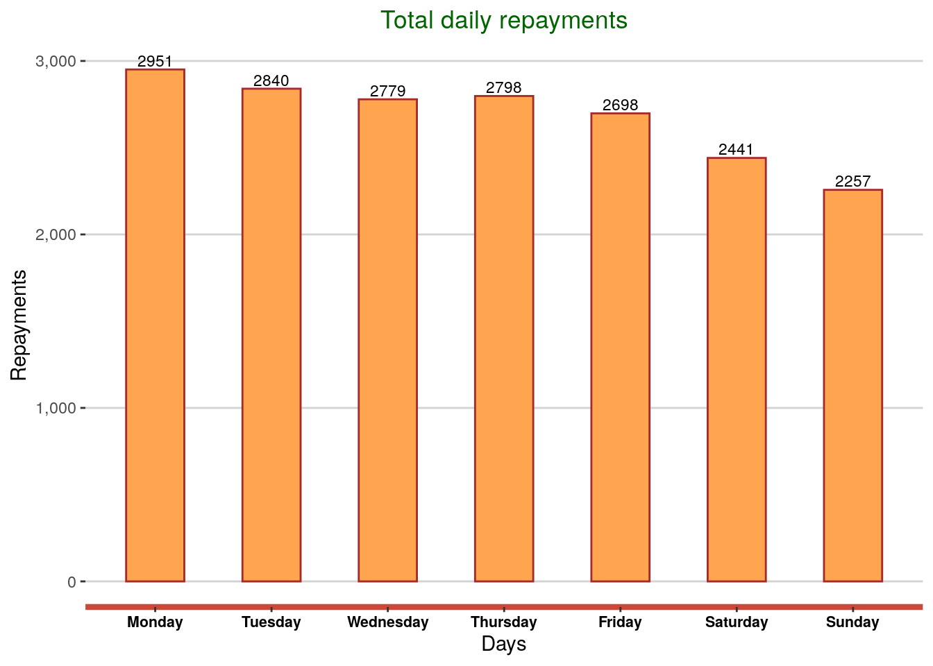
8.Daily loans repayment analysis
The Final repayment date was used to analyze for the repayment days. This analysis shows progressive loan repayments with days of the week. However, the difference in not much dispersed. Low repayments were observed over the weekend. Knowledge of repayment days will be very crucial when it comes to collection.
Shifting collection to the most likely repaying days will ensure proper resource allocation in terms of the number of messages to send in a week or number of customers to be contacted. Better still, if the repayments are low over the weekend, what strategies need to be put in place if the collection team is not working over the weekend? Curate and schedule specific repayment reminder messages on Friday evening?
#Generate weeks data
Week <- data %>%
  group_by(Product, `Final Payment Date`) %>%
  summarise(count = n())
 Week$`Final Payment Date` <-  as.Date(Week$`Final Payment Date`, format = "%Y-%m-%d")

 #change date into days of the week
 Week$day <- format(as.Date(Week$`Final Payment Date`), "%A")

 Week_plot <- group_by(Week, day) %>%
   mutate(Total = sum(count))


Week_plot <- Week %>%
     group_by(day) %>%
     summarise(sum(count))

Week_plot <- Week_plot[-c(8), ]

names(Week_plot) <- c("Day", "Total_Repayment")

Week_plot$Day <- factor(Week_plot$Day,
                        levels = c("Monday", "Tuesday","Wednesday","Thursday","Friday","Saturday","Sunday"))